Have you ever wondered which edge detection methods are best for given images? Yeah? So am I, so let's compare them.
We will be implementing some of the most commonly used methods and also using methods from OpenCV and PIL
We will be comparing the following methods:
- Sobel edge detector
- Prewitt edge detector
- Laplacian edge detector
- Canny edge detector
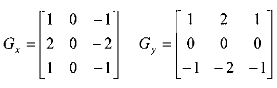
Sobel Operator
The sobel is one of the most commonly used edge detectors. It is based on convolving the image with a small, separable, and integer valued filter in horizontal and vertical direction and is therefore relatively inexpensive in terms of computations. The Sobel edge enhancement filter has the advantage of providing differencing (which gives the edge response) and smoothing (which reduces noise) concurrently.
Here is a python implementation of Sobel operator
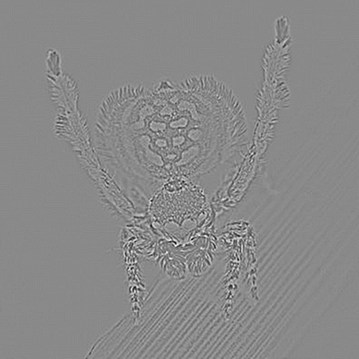
Results:
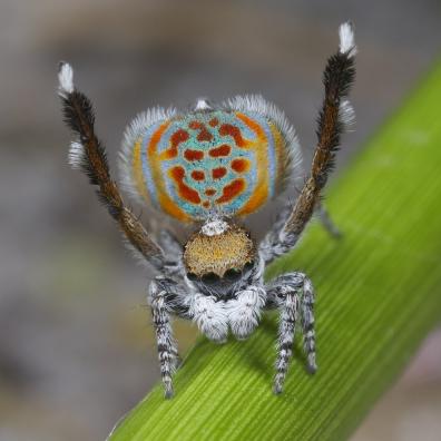
In this example we apply the mask on the gray-scale image, however we can produce a better result by applying the mask on each RGB channel.
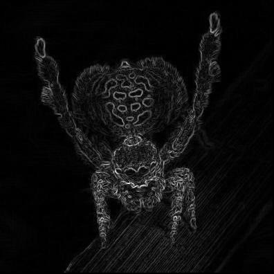
Results: One channel(left), RGB channel(right).
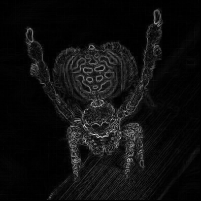
You can see a slight improvement but note that it's computationally more costly.
Prewitt’s Operator
Prewitt operator is similar to the Sobel operator and is used for detecting vertical and horizontal edges in images. However, unlike the Sobel, this operator does not place any emphasis on the pixels that are closer to the center of the mask.
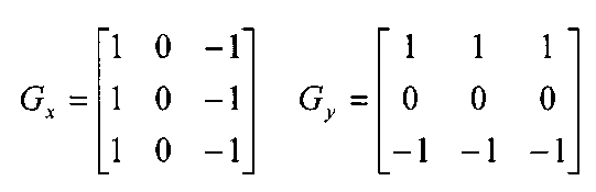
The only differance is the mask
Result:

Laplacian Operator
Laplacian is somewhat different from the methods we have discussed so far. Unlike the Sobel and Prewitt’s edge detectors, the Laplacian edge detector uses only one kernel. It calculates second order derivatives in a single pass. Two commonly used small kernels are:
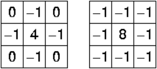
Because these masks are approximating a second derivative measurement on the image, they are very sensitive to noise. To correct this, the image is often Gaussian smoothed before applying the Laplacian filter.
We can also convolve gaussian mask with the Laplacian mask and apply to the image in one pass. I will explain how to convolve one kernel with another in a separate tutorial. However, we will be applying them separately in the following example. To make things easier we will be using OpenCV.
Results:
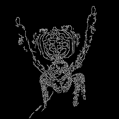
Canny Operator
Canny edge detector is probably the most commonly used and most effective method, it can have it's own tutorial, because it's much more complex edge detecting method then the ones described above. However, I will try to make it short and easy to understand.
- Smooth the image with a Gaussian filter to reduce noise.
- Compute gradient of using any of the gradient operators Sobel or Prewitt.
- Extract edge points: Non-maximum suppression.
- Linking and thresholding: Hysteresis
First two steps are very straight forward, note that in the second step we are also computing the orientation of gradients "theta = arctan(Gy / Gx)" Gy and Gx are gradient x direction and y direction respectively.
Now let's talk about Non-maximum suppression and what it does. In this step we are trying to relate the edge direction to a direction that can be traced along the edges based on the previously calculated gradient strengths and edge directions. At each pixel location we have four possible directions. We check all directions if the gradient is maximum at this point. Perpendicular pixel values are compared with the value in the edge direction. If their value is lower than the pixel on the edge then they are suppressed. After this step we will get broken thin edges that needs to be fixed, so let's move on to the next step.
Hysteresis is a way of linking the broken lines produced in the previous step. This is done by iterating over the pixels and checking if the current pixel is an edge. If it's an edge then check surrounding area for edges. If they have the same direction then we mark them as an edge pixel. We also use 2 thresholds, a high and low. If the pixels is greater than lower threshold it is marked as an edge. Then pixels that are greater than the lower threshold and also are greater than high threshold, are also selected as strong edge pixels. When there are no more changes to the image we stop.
Now let's looked the code:
Results:
If you have any questions or I messed up somewhere, please emails me at nikatsanka@gmail.com